GeoMx® DSP
Knowledge Base

Yes, you can scan your slides and select regions of interest (ROI) without collection using the “Scan only” feature. This feature is useful when evaluating tissue staining conditions prior to the experimental run, or practicing/discussing ROI selection prior to collection. When creating a new scan, one can toggle to select “Scan only” on the scan configuration window. Scans which are designated as scan only cannot be sent for ROI collection but can be transferred to Scan and Collect slide at another run using the ROI transfer function.

We do not recommend using TE buffer or any other buffers on the GeoMx DSP instrument, other than those provided in our instrument buffer kit. This is because the different salts could crystallize and clog the fluidic lines. Additionally, our reagents contain antimicrobial agents to prevent microbial growth, which may not be present in other buffers.

The GeoMx DSP instrument will rehydrate your slides every 4 hours, so they will not dry out. One caveat to this if the instrument errors out during collection, the slides will not re-hydrate. Also, the storage conditions inside the GeoMx DSP are not optimal, so we recommend that you remove them as soon as possible and store them according to the slide storage guidance within the GeoMx DSP Slide Preparation User Manuals (MAN-10150 and MAN-10151).

For protein slides, slides can be stored for up to 1 day submerged in 1X TBS-T and stored at 4°C, protected from light. For storage from 1 day to 3 months, the slides can be mounted with mounting media, mounted with coverslip, and stored at 4°C, protected from light.

For RNA slides, the slides can be stored for up to 6 hours submerged in 2X SSC and stored at room temperature, protected from light. Slides can be stored for up to 21 days in 2X SSC, at 4°C, protected from light. It may be necessary to re-fresh morphology marker or nucleic acid stain; please refer to our manual for guidance on this.

For GeoMx DSP Spatial Multiomics (formerly known as Spatial Proteogenomics) assay, store the slides in 1X TBS-T at 4°C, protected from light for up to 7 days.

For best results, minimize storage time between slide preparation and loading on the GeoMx DSP instrument while avoiding tissue from drying out.

Once the GeoMx DSP plate collection is complete, you can proceed to seal it with a permeable membrane and proceed to dry down the plate. To store the plate, seal it with adhesive foil to prevent contamination and store it at 4°C for 24 hours or less. For storage between 1-30 days, it can be stored at -20°C. For longer than 30 days, we recommend storing it at -80°C. Further guidance for this process can be found within the NGS Readout User Manual.

If you encounter a critical error during collection, please reach out to support.spatial@bruker.com to initiate a case. A support representative will send you a link to submit the instrument log files. To download logs, please go to the Administration tab within the GeoMx DSP Control Center on-instrument, followed by Download Logs.  In the custom range, select one day before the issue occurred to one day after, and in the “include images with download” option, choose “none”. You can then proceed to download the logs.

While the Support Team makes our best effort to respond in the same day, it is not always possible for us to do so. Therefore, to protect the samples, we recommend removing the slides from the instrument and safely storing them as outlined below, until the Instrument issue is resolved.

To retrieve your slides from the instrument:

• If you are logged in as an Administrator user, follow the steps below:
  • Under the Administration tab of the GeoMx DSP instrument, please select User Service Actions, select Home All to home instrument hardware. Then, select Control Door Lock, enter desired parameter: False = unlock door and True = lock door.
• If you are logged in as a General user, follow the steps below:
  • Under the Administration tab of the GeoMx DSP instrument, select System Settings, then the System Shutdown tab, then Shutdown System. Once the instrument is turned off, the door will unlock to allow you to remove your slides and collection plates.
  • If you do not have access to the holder at that time, please turn on the machine (this will home all motors) and turn off once again through the System Settings menu (to unlock the door). Allow at least 1 minute between reboots so that the software fully initializes.

Slide storage recommendations are as follows:

Protein – submerged in 1X TBS-T at 4ºC, protected from light.

RNA – submerged in 2X SSC at 4ºC, protected from light.

Spatial Multiomic/Proteogenomic Assay (RNA and Protein Assay on the same slide) – submerged in 1X TBS-T at 4ºC, protected from light.

It is possible to move GeoMx DSP scans and studies to and from any GeoMx DSP instrument using GeoMx instrument’s Data Exchange option. Simply export the GeoMx DSP scans and studies into external drives (NTFS format recommended and not greater than 10 TB) and then import into the other GeoMx DSP instrument using the Data Exchange option under the Administration tab. For detailed instructions on this, please refer to GeoMx DSP instrument user manual.

There are two types of user accounts on the GeoMx DSP instrument, administrator and general. Administrator has access to all the studies and full administration tab options, whereas a general user only has access to their own data. To create a new user account, please go to the Administration tab and select User Management. Here, you may create a new user.

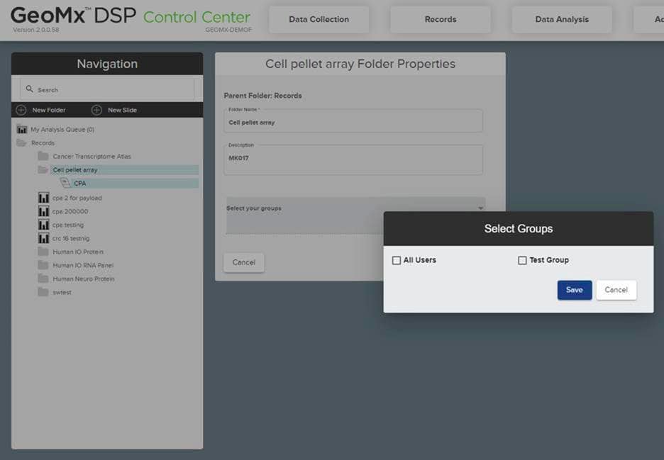
To assign users to a group, go to the Group Management option under Administration tab and click the “Manage” button to create a new group. From there you can check, add, or remove users as needed. Next, create a new folder and move files, scans, and studies into it by dragging and dropping and assign them to this group. To restrict access to the folder; right click on the folder, select “Edit” and then choose the group you want to grant access to the group. Please check the screenshots below for visuals on this:

With software version 3.0 and above, you can delete scans and studies from the GeoMx DSP instrument. This can be done by right clicking on the item’s name and then selecting delete to move this item to the trash folder. Using administrative level access, Scans can also be permanently deleted from the trash folder which will remove it from instrument and the archive. Please note that only scans with status Readout Complete, Scan Only, Error or Aborted can be deleted.

If you are not planning to run your GeoMx DSP instrument for 2 weeks or longer, we recommend running the hibernation protocol on your GeoMx DSP instrument to prevent any crystallization or salt accumulation in the lines. This protocol involves switching the buffers to DEPC-treated water and then flushing them. When you are ready to use the instrument again, it can be returned to operational status by following our protocol. Please refer to the GeoMx DSP Instrument user manual here for detailed instructions.

We do not recommend moving GeoMx DSP instrument on your own, even for a short distance. The reason is that the GeoMx DSP has a leveling process that is critical to its performance. Therefore, we highly recommend having our service engineer on-site to assist with move and post-move validation. Please reach out to customerservice.spatial@bruker.com to assist with this request.

This is possible in some cases; please refer to the table below. Note that this can only be done when the scan status is “Readout Complete.” To proceed, the user will need to complete all the steps including uploading RCC or DCC files. Then, from the scan gallery, click on “Scan Parameters” to update the probe kit files, and save the changes.

For NGS readout, user will need to download a new readout package and re-run the pipeline using the new configuration.ini file. The resulting DCC files can be uploaded to overwrite the original DCC files. For nCounter readout, creating a new study with this scan will show the updated counts.

The IPA panel consists of a core and IPA module. Thus, there are 2 .pkc files associated with this panel and both need to be added. Please note that the IPA Core kit must be selected before the compatible module kits will be available in the dropdown.

Also, configuration files are not pre-loaded on the instrument and must be transferred using a USB drive or remote access over Chrome. Probe kits for all panels can be found on our website here. We recommend uploading new .pkc files under Kit Management in the Administration menu. Once uploaded to the instrument, they are available for selection in the Scan Configuration window.

Windows Defender anti-virus is configured and will receive anti-virus definitions if the instrument has a network route to retrieve updates. In addition to using Windows Defender, we use Windows AppLocker. AppLocker is a whitelisting program that only allows NanoString-approved applications and processes to execute in Windows. As a result, AppLocker also provides robust protection from viruses and malware by blocking execution and enforces a high degree of overall change control of the DSP system state. In contrast to traditional security software that relies on blacklisting, which is inherently vulnerable to zero-day attacks and situations where the blacklist happens to not be updated in a timely manner, AppLocker blocks everything except the software/Apps that has been specifically allowed to run on the instrument. AppLocker allows us to maintain a static, robust, and secure application execution environment and protects the instruments from any unauthorized software or manipulation while at the same time ensuring that the machine remains in an unchanged and securely validated state.

There are three features that require network connectivity:

• Desktop clients access the web interface via the Google Chrome browser for remote ROI selection and data analysis.
• Establishing an automatic data backup system to the archiver server is strongly recommended. If no SMB backup location is established, the instrument will stop working when the hard drive is full. The instrument ships with a 10TB hard drive for OS and GeoMx DSP software installation and storage. On average, 20 GB per scan will be used for storage. At medium throughput, the instrument could run out of hard drive space after 6-8 months if no external storage is established. The effective storage can be expanded by allowing the instrument to connect to a corporate file share via SMB. When connected to external storage, the instrument will backup data to the network share.
• Bruker Spatial Biology includes remote support with the instrument, which allows for faster resolution of issues with the ability for Bruker Support to diagnose, configure, and update components remotely. To accomplish this, the Instrument must have WAN/internet access for Bruker Support personnel to access the instrument.

GeoMx DSP and auxiliary server need to have a static IP or reserved DHCP.

The best way to free up space is to connect to an archive server. This will move data from the instrument to the hard drive so that the instrument always has 2TB of free space. It will move the oldest studies/those that were opened the longest ago to the archive first. Please note that once you do set up an archive, the moving of data process is quite slow and could take several days. For more information on how to set up the archive drive, please refer to the GeoMx DSP Instrument user manual here.

Another way to free up some space is by deleting some scans and studies from the instrument. To delete old scans, you first need to move them to the trash and then an administrator user needs to go into the trash folder and delete them from the trash there. For more details on this, please refer to the GeoMx DSP Instrument user manual.

The maximum modules you can run include the Immune Cell Profiling Core, 6 human IO modules, and a custom module. Since both the immune cell typing and the MAPK module occupy the R4 space, you typically need to drop one human IO module to accommodate the MAPK module and use the substitute probe R for the hybridization step. However, if you prefer to run the immune cell profiling core with all the 7 human IO modules, that is feasible. In this case, MAPK module would need to be shifted to the R8 and R9 space and ordered from an external vendor such as Eurofins, IDT, etc. However, in this case, customers would lose the ability to add any more custom targets.

All nCounter readout products, whether RNA or protein, utilize the same DSP_v1.0 RLF and it should be installed on the Pro/MAX/FLEX or SPRINT during training. If not installed, please reach out to support.spatial@bruker.com to request the file.

The Hyb Code letter must match the Collection row letter. If an incorrect Hyb Code row number is used, we do not have a process to fix this error on a commercial scale. Therefore, it is crucial that the lab process be carried out exactly as described in the lab worksheet. You may collect a dummy ROI into wells and then finalize the row leading to the next collection starting in the next row. For instance, if you only have Hyb Code C on hand, you will need to do this dummy collection for rows A and B so that your actual samples will be collected into row C to match your Hyb Code C. Alternatively, you can order a new Hyb Code Pack for the collection.

This error is due to not uploading the hybcode lot specific files. You can resolve this issue by following these steps:

1. Locate your HybCode Box from -80C freezer, find the lot number written on the box.
2. Click on the 96-well plate icon on the GeoMx DSP screen (or where it says “No Plate”), and input the plate ID. Then, enter that Hyb Code pack lot number and click “update” – visuals and instructions here.
3. Download the calibration files associated with your lot and nCounter system here, leave them zipped!
4. Upload the calibration files to the GeoMx DSP instrument using the “Data Collection” -> “Upload Counts” button.

Once the calibration files are successfully uploaded, you should be able to upload your RCC files.

There could be several reasons to get an error while uploading the RCC files:

• Make sure there is no subfolder folder within the RCC.zip folder.
• Make sure the correct CDF was used for the nCounter run.
• Make sure SampleID in the CDF matches SampleID and CartridgeID in the RCC files.
• Make sure the correct Hyb Code Lot number is associated with the experiment. Check by clicking on the plate icon.
• nCounter data requires a calibration file for each new lot of Hyb Code. Please see the above question for further information on resolving this.

If you are still having issues, please reach out to support.spatial@bruker.com.

If only a few rows of the Seq Code plate were used, then you can use the remaining rows as long as the Seq Code plates are stored correctly. Also, it is important to match the Seq Code row with the collection plate row. Thus, you will need to enter the original collection plate number, so the instrument knows which row to start the collection (you may or may not use the same collection plate).

We do not recommend using the remnants of Seq Code for a second experiment. Because the Seq Code fill volume is 8 µL, it is possible the remaining volume will be less than 4 µL when reused. The extra volume can help salvage this step if a pipetting error occurs; otherwise, the wells contain single-use volume. You may however always use unused wells, please see the above FAQ on how to use the remaining wells of a Seq Code plate.

It is possible to move the collection plates from one readout group to the other one. For this to work, the collection plates must have the same status (eg. Finalized) to be moved to the same readout group.

In addition to this, the following combinations of plates are not allowed in one readout group:

• Single analyte plates using Pro Code indices (IPA) with single analyte plates using Seq Code indices
• Single analyte plates with mixed analyte plates
• Mixed analyte plates using Pro Code indices (IPA) with mixed analyte plates using Seq Code indices.

Steps to move plates from one readout group to another:

• Click on the plate icon on the GeoMx DSP instrument

• Enter the plate barcode number and then click on the readout group name in the window
• You then have the option to select MOVE

• Clicking on move will pull up a screen to select the collection plate to be moved from one readout group to the other.

• Click the Choose button and Readout Group window will appear

• Select the new Readout Group to assign to your plate and select Use Readout Group
• Your plate should be updated with a new Readout Group

For RNA assays with NGS readout, you need to have at least 4 ROI, otherwise the instrument will not allow you to finalize the plate. To resolve this, you can move this plate to a different readout group and then finalize them together. For more information on moving plates, please check the above FAQ How can I move collection plates from one readout group to another?

The readout package is a zipped folder that is downloaded after finalizing the collection plate for NGS readout. It contains 3 files:

• Configuration.ini file: this is the file used by the GeoMx NGS pipeline to assist in converting the Illumina FASTQ files to DCC files.
• Lab worksheet: contains information on the contents of each well of each plate, including ROI and segment details, ROI coordinates, scan details, biological target details, nuclei count, recommended sequencing depth, and more.
• Sample index list (SeqCodeindices.csv): this is the file needed to set up the Illumina sequencing run for demultiplexing the Illumina run (NextSeq 1000/2000 users download a SampleSheet.csv and whitelist.txt instead of an Indices.csv.)

To download the readout package:

• Click the bottom right corner of the screen. It should be a picture of a plate or say, “No Plate”. The Plate Information window will appear.
• Select the tab “Search by Readout Group”
• Click Look Up Readout Group and select the readout group that you want to export
• Enter/change the sequencing parameters and readout group information
• Insert USB drive
• Click “Finalize and Download Readout Package”. If the collection plate was finalized before, then you will see the option to “Re-download Readout Package”

Our recommendation for all Illumina instruments is to run GeoMx libraries at 2 x 27 paired end read strategy. We highly recommend Paired end workflow as it allows higher quality data, typically with no added kit cost.

We recommend assessing library quality on a capillary electrophoresis device such as the Agilent Bioanlayzer or similar to check amplicon size, concentration, and absence of contaminating primers. It is helpful to assess the library at stock concentration, in a dilution and checking the NTC library.

The expected library amplicon size is 162 bp (Seq Code products) or 166 bp (Pro Code products). Using the Bioanalyzer, the library will appear as ~150 bp. Using the TapeStation, the library will appear as ~ 170 bp.

Sequencing kits are sold per cycle. Since we recommend paired-end 2×27 read strategy, a sequencing kit that can accommodate at least 54 cycles (2 x 27 = 54) is required. The minimum number of cycles per kit for most Illumina sequencers is 75 or 100 cycles. In the case where customers are pooling DSP libraries with other Illumina libraries, then they must choose a kit that can accommodate the longest desired read length. Please discuss with your sequencing facility for more information on this.

The FASTQ files should always follow the standard Illumina naming structure:

DSP-PlateNumber, Seq Code plate letter, GeoMx Plate Well Number, sample sheet number, lane, read1/read2, always end in ‘001’

For example: DSP-1001250001985-A-A02_S2_L001_R2_001.fastq.gz The suffix .gz indicates a compressed (gzipped) file.

DSP-1001250001985-A-A02 is the “sample ID” matching that found in the configuration.ini and SeqCodeindices.csv files. A Translator file allows you to run the NGS Pipeline with FASTQ file names that are not an exact match to the configuration file sample name by translating one to the other. However, the translator is only useful for files with a different sample ID in the file name. All other elements – _S2_L001_R2_001.fastq.gz in the example above – must match the expected naming structure. If this is not the case, it will be necessary to rename the FASTQ files or request your sequencer to repeat demultiplexing following the above Illumina naming structure.

To use the translator file, please check here for the example file and instructions on how to use it.

For RNA or protein only assay, there is one fastq.gz file number per ended read (Read 1 “R1” and/or Read 2 “R2”) per flow cell lane (e.g. lane 1 “L1”, lane 2 “L2”, lane 3 “L3”, etc.)

For example, if a customer collects 133 AOI, then with paired end read strategy and run on 1 Flow cell lane, it will generate 266 FASTQ.

For GeoMx DSP Spatial Multiomics (formerly known as Spatial Proteogenomic) assay, there is one fastq.gz file number per ended read (Read 1 “R1” and/or Read 2 “R2”) per flow cell lane (e.g., lane 1 “L1”, lane 2 “L2, lane 3 “L3”, etc..) per analyte.

For example, if a customer collects 133 AOI, then with paired end read strategy and run on 1 Flow cell lane, it will generate 266 FASTQ for RNA and 266 FASTQ for protein, for a total of 532 FASTQ.

Yes, this is possible, but the files need to be merged at the level of the GeoMx NGS pipeline, because uploading another batch of DCCs with the same name to the GeoMx DSP instrument will just overwrite whatever is associated with that scan record.

To combine multiple runs, make sure that each set of FASTQ has a differing lane number (L001, L002, etc.) to allow the GeoMx NGS Pipeline to identify and merge them.

If necessary, it is possible to rename the files from multiple sequencing runs so that no two pairs of FASTQ share the same lane number. These renamed files can be run through a locally installed version of the GeoMx NGS Pipeline. These files cannot be uploaded to Illumina’s Basespace due to upload restrictions surrounding file naming and file metadata matching. It is not necessary to be concerned with whether the samplesheet number (_S4_) matches or not.

For example, we have two runs of a NovaSeq (1 lane) of the same library, which yields two sets of FASTQ:

DSP-1001250002271-A-A04_S4_L001_R1_001.fastq.gz

DSP-1001250002271-A-A04_S4_L001_R2_001.fastq.gz

DSP-1001250002271-A-A04_S32_L001_R1_001.fastq.gz

DSP-1001250002271-A-A04_S32_L001_R2_001.fastq.gz

Rename the second set so that L001 becomes L002, and put all files in the same root folder to process through the pipeline

DSP-1001250002271-A-A04_S4_L001_R1_001.fastq.gz

DSP-1001250002271-A-A04_S4_L001_R2_001.fastq.gz

DSP-1001250002271-A-A04_S32_L002_R1_001.fastq.gz

DSP-1001250002271-A-A04_S32_L002_R2_001.fastq.gz

All 4 files for sample DSP-1001250002271-A-A04 will be processed into one DCC file.

You cannot generate a dummy FASTQ file. However, you can run the standalone NGS pipeline (not Basespace) to generate an empty DCC file for the missing FASTQ. There may be a warning message that it is missing some inputs, but once proceeded the pipeline will create an empty DCC file of size ~ 1kb for the missing FASTQ.

The GeoMx NGS Pipeline uses a series of algorithms to process sequencing files from FASTQ to the Digital Count Conversion (DCC) file format that can be read by the DSP instrument for further analysis. First, raw sequencing files (FASTQ files) are selected for a specific pipeline run. Once selected the reads are processed for quality, the adapters are removed (trimmed) and the paired-end reads are merged (stitched) resulting in a single high quality read. Then, reads are aligned to the Readout Tag Sequence-ID (RTS-ID) barcodes. PCR duplicates are removed by matching on the Unique Molecular Index (UMI) (deduplicated) and the DCC file is generated. The resulting DCC files are presented as a .zip file in a folder which you designate and can then be uploaded into the DSP Control Center for study creation in the DSP Data Analysis Suite.

It can be run two ways:

• Install NGS Pipeline Software on a computer server
• Use BaseSpace Sequencing Hub’s cloud pipeline application, called DRAGEN

Refer to the GeoMx DSP NGS Readout User Manual (MAN-10153) for more information.

The following can be checked to ensure there are no issues while uploading the DCC files into the GeoMx instrument:

• Make sure the folder is zipped (must be .zip).
• Make sure there is not a subfolder within the zipped folder.
• Make sure there is a DCC file for every sample in the readout group

If you are still having issues, please email support.spatial@bruker.com.

This error comes up when the DCC file is missing the umiQ30 field. Usually, when a FASTQ file is missing for one of the AOI/ROI, the pipeline generates an empty DCC file that helps the user to upload and reach readout complete status for their scan with 0 counts for that AOI/ROI. Presently, when a user uses DRAGEN pipeline on Basespace, a bug causes certain header fields to be filled incorrectly. The instrument cannot parse these DCCs at upload and throws an error. You can recognize this issue by looking in the DCCs and checking the <NGS_Processing_Attributes>:

Bad

Good

Just edit the incorrect file, zip together with the other DCC files, and then try to upload the data again. If you are still having issues, please email support.spatial@bruker.com.

You can upload DCC files again and the data will be replaced by the latest uploaded ones. After you upload DCC files, any studies already created will not be updated, but any new study will use the latest counts.

The UV cleaving area can resolve a single cell. However, 5,000 oligos per target are required for analysis of a given ROI. This translates to 2,500 bound antibodies and 250 RNA molecules per ROI. Therefore, we suggest a minimum of 20 cells in each region of interest (ROI) for protein analysis and 100 cells for RNA analysis. Signal is proportional to collected mass, therefore selecting smaller ROI may result in lack of signal.

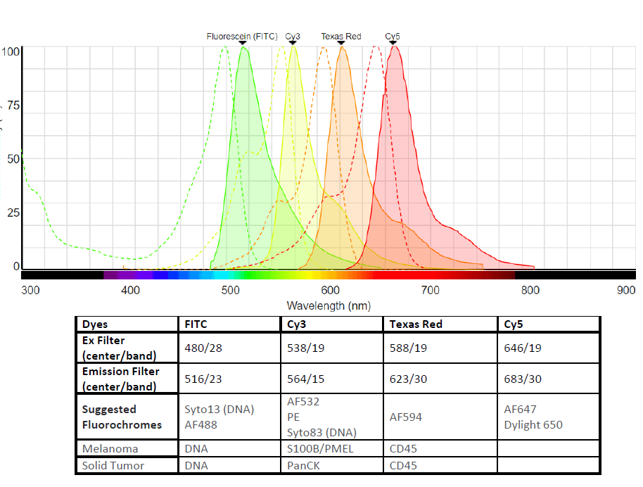
Four fluorescent channels are used. Representative dyes include FITC (AF488), Cy3 (AF532), Texas Red (AF594) and Cy5 (AF647).

Yes, it is possible to analyze both protein and RNA expression from individual Area of interest (AOI) on a single slide with up to 18,000 RNA targets and 570+ protein targets across dozens of pathways using GeoMx DSP followed by NGS readout on an Illumina sequencer. For more information on the Spatial Multiomics (formerly Spatial Proteogenomics) workflow, please check out our white paper explaining the entire workflow as well as our manual.

The safest option is to run GeoMx DSP and H&E staining separately, performed using serial sections. If you want to run them on the same slide, then please run the GeoMx DSP workflow first, followed by the H&E staining for histotyping. This strategy has been successful with our internal team for protein slides.

GeoMx DSP works with positively charged slide mounted with 5 µm FFPE tissue sections. It has been validated for fresh frozen as well as fixed frozen samples (Appendices II and III, respectively, in the GeoMx Slide Prep User Manual). Additionally, tissue microarray samples can also be analyzed if the sections are within the recommended scan area (see the green area in the figure below) and at least 2-3 mm apart.

FFPE samples should be fixed with 10% NBF or 4% PFE and embedded in paraffin. We recommend 18-24 hours fixation time for blocks less than 0.5 cm in thickness. The paraffin blocks can be stored long term for future use on GeoMx DSP. Fresh/frozen tissue should be stored in optimal cutting temperature (OCT) media. After sectioning on a cryostat, user can follow the instruction in the manual for either the FFPE or fresh frozen/fixed frozen workflows.

GeoMx DSP is fully validated for samples up to 3 years old prepared from tissue with a cold ischemic time of less than 1 hour using 10% NBF or similar fixative.

Internally, we have tested up to 40-year-old blocks. For 10- to 20-year-old blocks, we have had good signal for RNA. For the 40-year-old block, the signal was low for RNA. Age is not the only consideration here. Cold/warm ischemic time, fixation, storage, etc. all play major roles. For the best results, do not use FFPE blocks that are more than 10 years old.

For GeoMx RNA assays, it is preferable to cut sections within 2 weeks of the time of running samples as oxidation of the RNA molecules begins shortly after cutting the section. Cut sections should be stored at 4° C with a desiccant pack. RNA quality is important for GeoMx DSP experiment with the RNA panel. RNA may be degraded in old sections, especially the low expressors. If concerned about the RNA quality, in situ hybridization or RNAscope can be performed on these samples and if there is good signal for low or middle expressors, then samples are okay to use for GeoMx DSP experiment. Please see the direct link to ACD’s control probe options. The most common kit for qualifying samples prior to GeoMx DSP is the RNAscope 3-plex positive control kit that matches the species (please see human here).

Protein is less sensitive to age, preservation, and storage conditions than RNA and customers may find a higher success rate for protein analysis on older blocks.

Bruker Spatial Biology recommends using positively charged slides. Internally, we have had the most success using Superfrost plus or Leica BOND plus slides (Catalog No. S21.2113.A). Although not validated by Bruker Spatial Biology, products like Epredia™ Tissue Section Adhesive (Fisher Scientific, Catalog No. 86014) or TOMO® Adhesion Microscope Slides (VWR, Catalog No. 10000-038) may also work well.

Citrate buffer and TRIS-EDTA both work with RNA assay; however, the number of targets below the LOQ is high when using citrate buffer for RNA assay. This is one of the steps that was extensively tested by our R&D team, hence our recommendation has always been to use TRIS-EDTA and not deviate from it for RNA work.

For our assays, the critical requirement for the water is that it is nuclease-free and RNase-free. Both DEPC-treated and nuclease-free water sources should meet these criteria and can be used in the GeoMx DSP workflow. (While DEPC can impact downstream enzymatic activity, most commercial DEPC-treated water is tested for inactivity post-treatment). Please note that the Spatial Multiomics (previously Spatial Proteogenomics) assay workflow calls specifically for nuclease-free water in the preparation of 1X TBS-T, not DEPC-treated water.

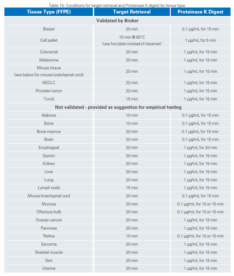
For RNA assays, the target retrieval conditions, and the Proteinase K digestion conditions vary among tissues. Our internal team has tested some tissues and shared the conditions that worked, highlighted below and printed in the GeoMx DSP Manual Slide Prep User manual. Target retrieval and Proteinase K conditions were determined based on FFPE tissue blocks meeting the constraints outlined in the sample guidance section of the GeoMx DSP Manual Slide Prep User manual. Samples were primarily tumor, with minimal normal adjacent tissue. These conditions may vary by sample, the amount of normal adjacent tissue, and other factors. These conditions were optimized for large tumor sections and may not apply to arrayed tissues, cored tissues, and needle biopsies.
Please note that if your tissue of interest is not mentioned here, we recommend using default conditions for the target retrieval (15 min at 100°C) and Proteinase K digestion (1 ug/mL at 37°C) steps.

Morphology markers are used by researchers to reveal tissue structures which are relevant to the research questions by helping to select regions of interest (ROI) and if desired, ROI segmentation into cell-type compartments. Directly conjugated primary fluorescent antibodies is the most straight forward approach. Bruker Spatial Biology offers several morphology marker kits for the commonly used markers. In addition, our internal teams have compiled a list of markers that have been used successfully internally, which can be accessed here. If conjugated antibodies are not an option, one can choose alternative approaches such as using antibody conjugation kits, secondary antibody staining protocol, as well as RNAscope for RNA assay. For more information on these approaches, please refer to our tech note on morphology markers here.

GeoMx nuclear staining kit includes a DNA dye (SYTO13) which is detected in the FITC/525 nm channel. You may consider using a different SYTO DNA dye (SYTO 83 and SYTO Far Red; sold by Thermo Fisher Scientific) to free up the FITC or Cy3 channels for other markers, if required. We do not recommend using DAPI for DNA staining for GeoMx DSP experiments. This is because UV light, which is required for DAPI excitation, is reserved for barcode cleavage.

For our Morphology Kits, the antibodies in the protein-compatible and the RNA-compatible kit are the same (exception: human CD45 antibody is different between RNA and protein kits) but in a different concentration. The antibodies in the RNA-compatible kit are 2X the concentration of those in the protein-compatible kit, so that the final concentration on the tissue is 2X compared to the protein-compatible antibodies. This is to compensate for the differences in slide prep methodology in the protein and RNA workflows. Therefore, you can use the Protein-compatible morphology markers with your RNA samples, please just use twice the starting amount of antibody when preparing your solutions for the slides.

Bruker Spatial Biology has observed the best tissue adherence with Leica BOND Plus slides and they are the preferred slide type for tissues with known poor adherence. In addition to this, extending the baking time to 37°C overnight followed by 65°C 3-4 hours may also help. For both the CosMx SMI and GeoMx DSP workflows, adjustments to the high-temperature antigen or target retrieval step may help preserve tissue adhesion. Fat-rich tissues, such as breast cancer, may benefit from shorter incubation times to avoid complete loss of adipose tissue. Delicate tissues and cell pellets may benefit from lowering target retrieval temperatures. Consult the Slide Preparation User Manual or the above FAQ on Target Retrieval and Proteinase K conditions.

The Spatial Multiomics (formerly Spatial Proteogenomics) assay could be performed manually instead of semi-automated BOND RX/RX workflow. The standard RNA slide preparation protocol in the GeoMx DSP Manual Slide Preparation user manual should be followed up to the Proteinase K digestion step, however, please use 0.1 µg/mL concentration instead of 1 µg/mL concentration. After the digestion step, the rest of the workflow can be followed as in the Spatial Proteogenomic Assay User Manual. (This workflow may also be referred to as Spatial Multiomics). Please note that this is not validated by Bruker Spatial Biology, thus some empirical testing may be needed on your end.

For GeoMx DSP assays with nCounter readout, you can spike in 5-10 targets of your choice.

For GeoMx DSP assays with NGS readout, protein panels such as GeoMx IO Proteome Atlas can accommodate spike in of up to 40 targets. For RNA assays with NGS readout, you can spike in up to 400 targets, which would have to be split into two 200-target spike-in add-on panels. In addition, customers can also design a standalone panel of only 200 targets with an additional 200 targets as add-on.

• WTA + 200 add-on + 2nd 200 add-on
• Standalone 200 + 200 add-on

Unfortunately, due to the complex nature of miRNA, we do not currently have a method to detect microRNA on GeoMx DSP.

We can design probes to detect circRNAs; however, to specifically detect a circRNA, we need to design the probe to straddle the back splice junction, and as a result, we can only get one probe for each circRNA. Therefore, there may be some sensitivity issues with these targets. In addition, since we have not validated circRNA detection, we would recommend including robust controls to assess the specificity of the probes.

Storage and shelf life for the GeoMx DSP reagents can be found in the table below. Storage conditions for GeoMx DSP reagents are listed on the individual reagent container as well as in the GeoMx DSP Slide Preparation user manual. These conditions include room temperature, 4˚C, -20˚C and -80˚C. Please read labels carefully to ensure correct storage and product integrity.

All GeoMx DSP reagents have a shelf-life of at least 1 year from date of manufacture, and for most items, the shelf life is 2-3 years from date of manufacture. Bruker Spatial Biology guarantees that products will have at least 3 months’ shelf-life remaining upon shipment.

To determine the expiration date of a reagent, please refer to the reagent packaging, which will show the date of expiration or the date of manufacture. The date of expiration is indicated by the hourglass symbol

and indicates the use-by date. The date of manufacture is indicated by the manufacturer symbol

and indicates the date the product was manufactured; refer to the table below for the shelf-life of the reagent from the data of manufacture.

Reagent	Shelf-life from Date of manufacture	Storage Temp
Slide Prep Reagents Buffer W	1 year	4°C
Buffer S Buffer R (RNA kit only)	3 years 1 year	4°C or RT 4°C
Morphology marker kit	2 years	4°C
Nuclear stain	2 years	-20°C
Instrument Buffer	3 years	RT
Collection Plates	No expiration
nCounter Readout
Protein Detection Kit Antibody Mix Probe Rs	3 years 5 years	-80°C -80°C
RNA Detection Kit	3 years	-20°C
Hybcode Pack	3 years	-80°C
GeoMx Hybridization Buffer	2 years	RT
NGS Readout
RNA Panels (eg. CTA, WTA, etc)	3 years	-20°C
Protein Panels (eg. IPA)	2 years	-80°C
SeqCode Plates	2 years	-20°C
ProCode Plates	2 years	-20°C
5X GeoMx NGS Master Mix	2 years	-20°C

Seq Code and Pro Code plates should be stored at -20°C. Once thawed, the plates can be stored up to 3 months at 4° C. Alternatively, the plates may be re-frozen and can go through up to 3 freeze-thaw cycles.

Safety Data Sheets (SDSs) can be found through the Resources page on our website or directly from the Bruker Spatial Biology home page under Support and Resources > Product Support > Safety Data Sheets. You may choose GeoMx DSP under instrument category to find the SDS specific to this instrument.

GeoMx DSP is paired with Data Analysis (DSPDA) software that allows users to easily visualize their data and simplifies data interpretation for both nCounter and NGS readout, covered in detail in our data analysis user manual here. Alternatively, users trained in R may extract their data and analyze it independently using open-source tools (Bioconductor). We also offer our Spatial Data Analysis Service (sDAS) for those who need further support. For more information on this, please check here.

Users can upload the RCC or DCC files to the GeoMx DSP instrument without the auxiliary server. Depending on the number of slides/AOIs, the data analysis steps may be executed slowly. Generally, nCounter readout panel data, CTA data, and WTA data from up to 4 slides can be analyzed on DSPDA without the need for an auxiliary server.

It is possible to do data analysis while doing data collection, however, this may overwhelm the software of the instrument and thus, it is recommended to wait for the run to complete and then perform data analysis.

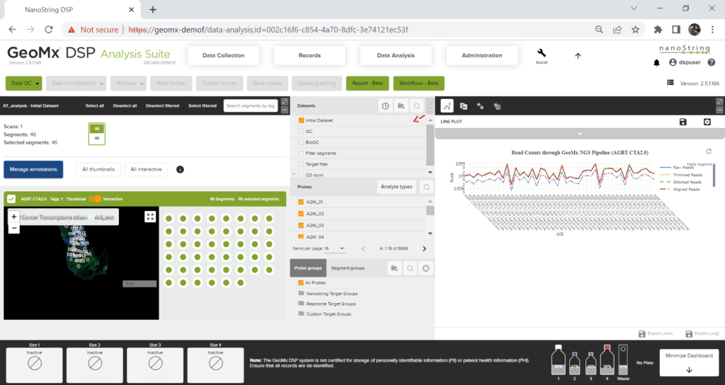
To download the initial dataset, open the DSPDA control center and in the Datasets window, hover over the right side of “initial dataset”. The save option pops up and the dataset can be saved as an Excel sheet.

You can find the X and Y coordinates in the initial dataset Excel file. For instructions to download it, please refer to the above FAQ. The X, Y coordinates are the center of your ROI as measured from the top left corner of the raw TIFF image. If your goal is to use the X, Y coordinates for plotting and if you are familiar with R, then we would recommend using the SpatialOmics overlay package available at GeoScripthub.

To download the GeoMx image, open the scan in the GeoMx DSP Scan Workspace. From the Export tab, select OME.TIFF and click export. This will export a multi-channel, pyramidal .TIFF images with ROI and Segment mask layers embedded in the header. For more information on this, please refer to our technote here.

• During scan setup, you may choose to select to include a No Template Control (NTC) well in the experiment, which receives no collection aspirate and therefore serves as a negative control during library prep/PCR amplification. The NTC may be used qualitatively, but it should not be used for data analysis correction.  It is normal to see raw sequencing reads (in FASTQ files), or relatively small numbers of final probe counts of any NTC well(s) compared to true sample wells. Generally, ensure that there are significantly more counts in experimental sample collection wells than the NTC and then move on.
• In the case of a high NTC that matches or exceeds counts from experimental sample collection wells, for a given plate, data analysis can proceed if the samples pass biological QC. If biological QC fails, then look at the NTC counts more closely. NTC counts are a good indicator of library prep cleanliness which depends on factors such as molecular biology technique, operator experience, lab SOPs, etc. If the NTC counts are high or increasing over time, revisit these factors for best practices or cleaning.
• NTC counts may be used qualitatively to indicate potential contamination but should not be used quantitatively, e.g., as an alternative background noise threshold for specific probes or panels. This is because contamination is not likely to be consistent across all wells in a plate.

Normalization is a data transformation that balances the results between segments within an analysis using the counts from a specific set of probes.

For NGS readout, Q3 normalization is the recommended normalization for RNA assay and geomean of housekeepers or isotype controls is the recommended normalization method for protein assays. For more information, please refer to the white paper Introduction to CTA: Normalization.

For nCounter readout, housekeepers and isotype controls are commonly used to normalize RNA and protein data. For more information on normalization, please refer to the white paper: Introduction to GeoMx Normalization.

We do not recommend checking your GeoMx data on nSolver as nSolver is not designed to handle any of the GeoMx panel data. The best way to analyze GeoMx data is on DSPDA or through R independently.

Yes, you can analyze your GeoMx DSP data from nCounter readout in R. However, you cannot do this directly using the RCC files since this data must first be demultiplexed and calibrated for reagent lot. If you wish to analyze your nCounter readout with R, please upload your RCC files into the DSPDA suite, create a new study and then download the initial data set. For instructions on how to download the initial dataset, please check the FAQ: How can I download the initial dataset? The initial data set could then be used to run on R independently.

The following files are needed to run on GeomxTools for NGS readout:

• DCC files
• PKC files (can be accessed here)
• Annotation files derived from the lab worksheet

For the Spatial Multiomics (formerly known as Spatial Proteogenomics) assay, there is only one configuration file for the entire WTA+IPA run. The config file and resulting DCC file names show only the SeqCode label; however, it does contain data for both RNA and protein analytes provided that all necessary PKC files were associated with the scan at finalization. Once the DCC files are uploaded to the instrument and the initial dataset is generated, quality control and subsequent data analysis steps are performed for each analyte separately, and datasets are distinguished in the DataSets pane by an analyte icon.

GeoMx DSP researchers can submit their data to the GEO database. Here is the webpage with all the relevant information on this.

For NGS readout, files to be submitted to GEO for publication include:

• Raw data files (FASTQ)
• DCCs
• PKC
• Metadata.xlsx

For raw data, most customers submit the FASTQ files.

For nCounter readout, the data should be submitted as other data types: generic single channel submission, including the following files:

• RCC files
• PKC
• Metadata.xlsx

For metadata, you can download the latest template from GEO here.